
In April 1997, the Japanese government raised the national consumption tax from 3% to 5%. The tax hike was implemented during recovery following Japan’s asset bubble collapse in the early 1990s. The asset bubble collapse left the economy stagnated with rising government debt. Japan’s government debt rose from 63% of its GDP in 1991 to 107% of its GDP in 1997. The consumption tax hike was implemented to combat the rising government debt burden. This fiscal policy primarily affects aggregate demand. A higher consumption tax raises the prices of goods and services which lowers household consumption and disposable income. This shifts the aggregate demand (AD) curve down and to the left.

AD-AS: In the AD-AS model, the consumption tax hike reduces consumption and overall demand in the economy, shifting the aggregate demand curve leftward (AD → AD′).
From the graph, the economy moves from the initial equilibrium at (P1, Y1) to a new short-run equilibrium at (PSR, YSR). Output falls (Y1 → YSR), and the price level also declines (P1 → PSR), reflecting reduced demand.
Because output falls below the natural level (YLR), there is a recessionary gap. Over time, as wages and expectations adjust, the economy moves toward the long-run equilibrium at a lower price level (PLR) while output returns to YLR or Y1.

IS-LM: The same fall in consumption that shifted AD left now shows up in the IS–LM model as a leftward shift of the IS curve (IS → IS′), since consumption and aggregate expenditure has decreased.
At the original price level, this shift leads to a new short-run equilibrium with lower output (Y1 → YSR) and lower interest rates (r1 → rSR). The fall in income reduces demand for money, which puts downward pressure on interest rates.
However, as seen in the AD–AS model, the price level is also falling (P1 → PSR → PLR). This increases real money balances (M/P), shifting the LM curve to the right over time. This partially offsets the decline in output, but not enough to fully reverse it.
The resulting lower level of output feeds directly into the labor market.

Labor Market: In the labor market, the fall in aggregate demand reduces firms’ need for production, decreasing labor demand. This is shown as a movement along the labor demand (LD) curve, leading to a decrease in employment from N1 to NSR. At the same time, the decline in the price level increases real wages in the short run (since nominal wages are sticky), moving from (w/p)1 to (w/p)SR.
Higher real wages make labor more expensive for firms, reinforcing the decline in employment. The short-run equilibrium therefore features lower employment and higher real wages, before adjustments gradually move the economy back toward long-run equilibrium.
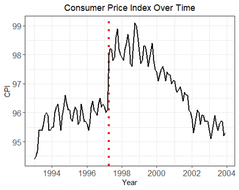
These model predictions are reflected in the real-world data. The CPI graph shows an initial increase in prices around 1997, driven by the tax itself raising the cost of goods. However, this is followed by a steady decline in prices over time.
This pattern suggests that while the tax mechanically increased prices at first, the underlying effect was a sustained decrease in demand, leading to deflationary pressure. Japan subsequently entered a recession in the late 1990s, often referred to as part of the “Lost Decade,” consistent with the fall in output and employment predicted by the models.
This pattern suggests that while the tax mechanically increased prices at first, the underlying effect was a sustained decrease in aggregate demand, leading to deflationary pressure. This aligns with the AD–AS model prediction that a leftward shift in AD reduces output and prices in the short run.
The fact that prices fall after the initial increase highlights a limitation of the model: it does not fully capture the difference between one-time price level changes (from the tax) and ongoing demand-driven inflation.
Additionally, Japan entered a recession in the late 1990s, often referred to as part of the “Lost Decade,” which is consistent with the predicted fall in output and employment. This suggests that the contractionary effects of the policy were stronger than intended.
Overall, while the model correctly predicts the direction of long-run effects (lower demand and falling prices), the real-world data shows a short-term price spike followed by deflation, indicating that incorporating policy timing and short-run price shocks would improve the model’s accuracy.
Simultaneous Shocks: In 1997, Japan experienced the Asian Financial Crisis which contracted aggregate demand even more. Furthermore, Japan’s banking sector also felt heavy distress due to debt accumulation from the asset bubble collapse a few years prior. This tightened credit availability and reduced investment and consumption beyond what the tax hike alone would have caused.
In April 2013, the Bank of Japan launched Quantitative and Qualitative Monetary Easing (QQE). The policy was implemented in response to 15 years of deflation and stagnant growth following Japan’s asset bubble collapse and the prolonged effects of the 1997 recession. The BOJ had already cut interest rates to near zero and implemented conventional quantitative easing, but neither succeeded in ending deflation. QQE aimed to double Japan’s monetary base within two years by purchasing massive amounts of government bonds and other assets, with the goal of reaching a 2% inflation target. The goal was to lower interest rates, encourage borrowing, and increase spending and investment. At the same time, the policy also aimed to influence inflation expectations by committing to continued monetary expansion until inflation not only reached but stayed above the target. This monetary policy primarily affects aggregate demand. An increase in the money supply shifts the LM curve to the right, lowering interest rates and boosting investment and consumption, which shifts AD to the right.
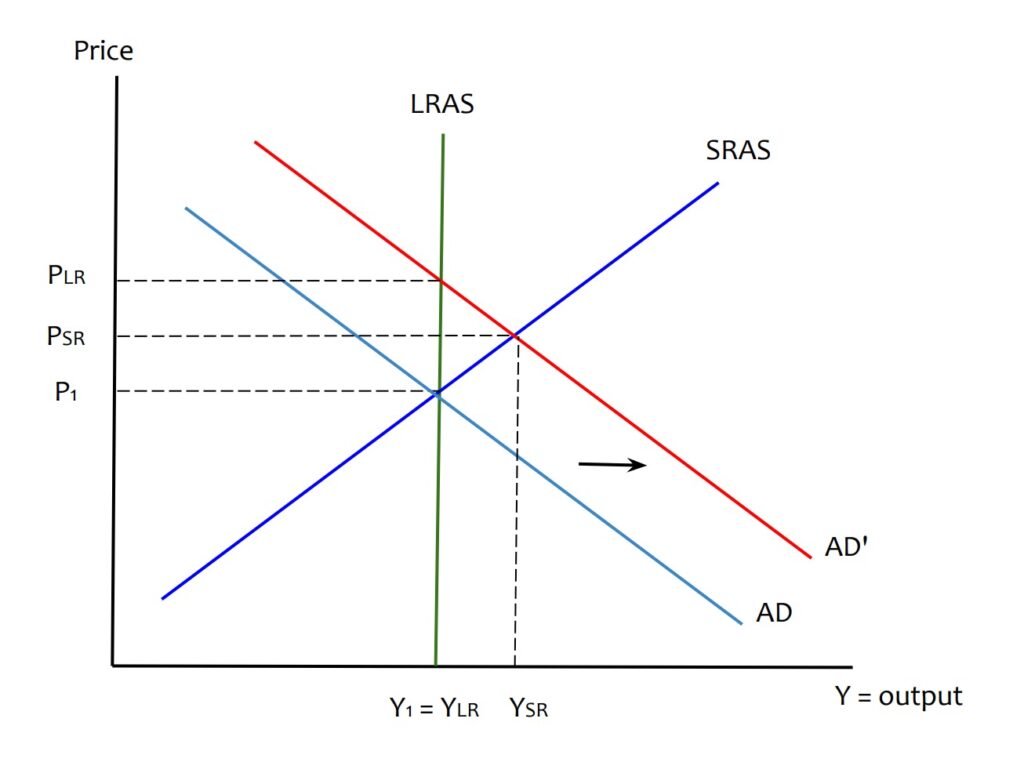
AD-AS: With more money (M) in the economy and lower interest rates, consumption and investment increase. This shows up in the AD–AS model as a rightward shift of aggregate demand (AD → AD′).
We observe this in the graph, as this moves the economy from the initial equilibrium to a new point with higher output (Y1 → YSR) and a higher price level (P1 → PSR). This helps Japan move out of its deflationary state.

IS-LM: The initial equilibrium occurs at the intersection of the IS curve and LM(M1, P1), with output at Yn and interest rate at r1. When QQE is implemented, the money supply increases from M1 to M2, which shifts the LM curve to the right from LM(M1, P1) to LM(M2, P1). At the same price level, this shift leads to a lower interest rate and higher output, moving the economy to the right along the IS curve.
As output increases, the price level rises from P1 to PSR, which reduces the real money supply (M/P). This causes the LM curve to shift slightly back to the left, from LM(M2, P1) to LM(M2, PSR). The final equilibrium is at the intersection of the IS curve and LM(M2, PSR), where output increases from Yn to YSR, and the interest rate settles at rSR, which is lower than the initial rate but higher than it would have been if prices had remained constant.

Labor Market: The initial equilibrium in the labor market is at employment N1 and real wage (w/p)1. As QQE increases aggregate demand and raises output, firms need to produce more, which increases the demand for labor. This is shown as a movement along the labor demand (LD) curve, increasing employment from N1 to NSR.
At the same time, the rise in the price level (from P1 to PSR) reduces the real wage (w/p) in the short run, moving it from (w/p)1 to (w/p)SR. This lower real wage makes it cheaper for firms to hire workers, reinforcing the increase in employment.
As a result, the new short-run equilibrium is at a higher level of employment NSR and a lower real wage, before eventually adjusting back toward the long-run equilibrium.
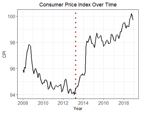
Shinzo Abe’s plan to expand monetary policy in 2013 does have some inflationary effects. We can see that the CPI does increase from a stable level at 94.5 to 95.5 in April of 2013 when his monetary policy comes into effect. This is followed by a further increase in price in the long term from 95.5 to 98 points a few months after. Thus, an increase in monetary policy does result in an increase in price just as theory had predicted.
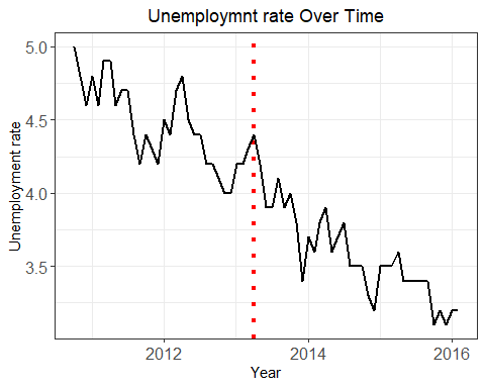
We also see models rightfully predicted a decrease in unemployment rate in the short run. However, real life data diverges in the long run where we continue to see the unemployment rate decrease, instead of increasing to its original level, this is likely because of macro-trends in the 2010s where we see the unemployment rates continuously decrease until 2020.
Simultaneous Shocks: While our models attribute Abenomics as the monetary policy aspect, it also included fiscal stimulus and structural reforms. Isolating the effect of QQE alone is difficult because there were other policies involved which affected aggregate demand as well.
Shortly after the implementation of QQE, Japan raised the consumption tax from 5% to 8% in April 2014. This could be a reason for CPI steadily increasing after QQE was enacted and not merely monetary policy driven.
Characteristics not captured in the model: The AD-AS model assumes a fixed natural rate of unemployment, but Japan’s aging population and shrinking labor force were gradually weighing it down throughout the 2010s. This could explain why unemployment kept decreasing after QQE rather than returning to previous rates. If we shift the natural rate of unemployment over time, we could better capture this trend.
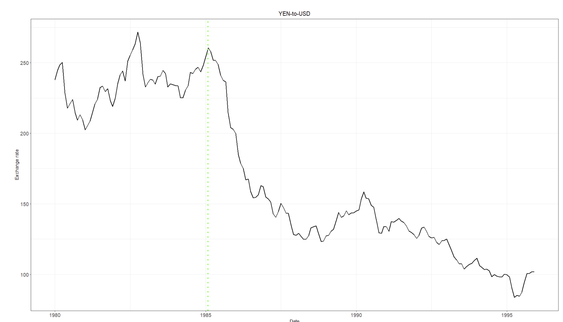
Figure 1: The appreciation of the yen after the 1985 Plaza Accord – represents the key global shock that set the stage for Japan’s asset price bubble.
The green lines indicates when the Plaza Accord is implemented.
This graph shows the exchange rate between the Japanese Yen and the U.S. dollar, where the yen strengthened significantly against the U.S. dollar. As the yen appreciated, Japan’s exports became less competitive, causing economic slowdown and disinflationary pressure. In response, the Bank of Japan adopted expansionary monetary policy by lowering interest rates to stimulate demand. This policy shift created the initial conditions for increased borrowing, credit expansion, and the eventual rise in asset prices.
Dataset source: fred.stlouisfed.org
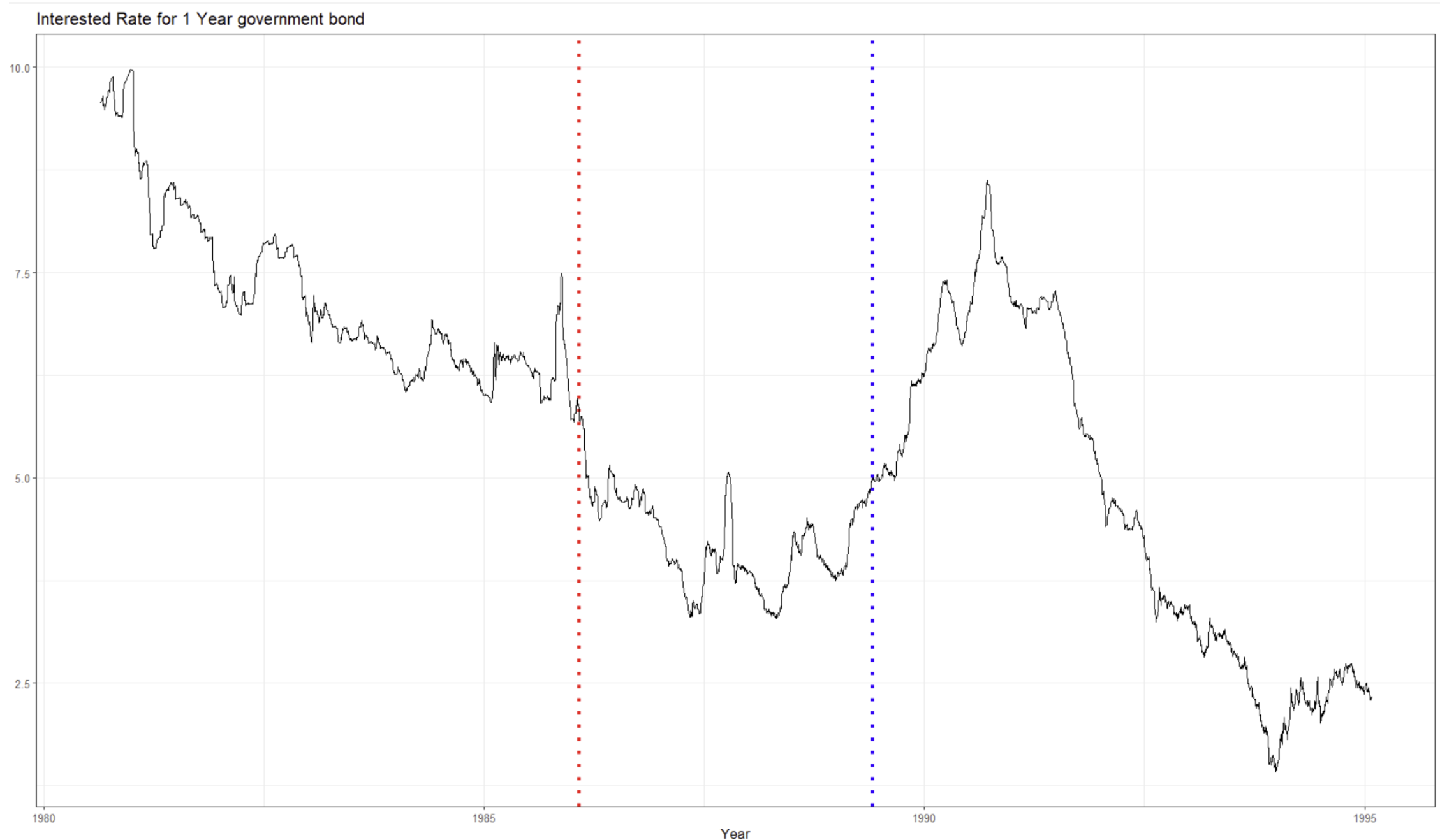
Figure 2: Interest rate movements during the late 1980s illustrate how expansionary monetary policy fueled the asset bubble and how later tightening contributed to its collapse.
This graph captures the dynamics of the interest rate; The red line is where the bank officially starts to reduce interest rate, and the blue line is where they officially start to raise the interest rate. Between 1985 and 1987, interest rates declined significantly, supporting money growth of around 8% and making borrowing cheaper. This encouraged firms and households to take on debt, often using real estate as collateral, which fueled speculative investment in asset markets. As borrowing increased, asset prices rose rapidly, creating a self-reinforcing cycle of speculation. In 1989, the Bank of Japan raised interest rates to control the bubble, increasing borrowing costs and tightening credit conditions. This shift marked the turning point, leading to a sharp decline in asset prices and the eventual bursting of the bubble in 1991–1992.
Dataset source: https://www.stat.go.jp/data/cpi/2020/kaisetsu/index.html
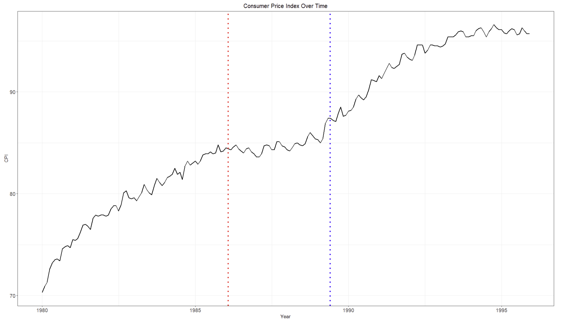
Figure 3: Consumer price inflation (CPI) remained relatively stable despite the asset bubble and its collapse, highlighting underlying disinflation and weak demand in the Japanese economy.
This graph shows the economic conditions of inflation; The red line is where the bank officially starts to reduce interest rate, and the blue line is where they officially start to raise the interest rate. Even as asset prices rose and later collapsed, CPI inflation remained relatively moderate, reflecting the absence of strong demand-side pressure in the broader economy. After the bubble burst, disinflationary and eventually deflationary pressures became more pronounced as investment and consumption declined. This indicates that while asset prices experienced extreme volatility, standard inflation measures did not capture the buildup of financial instability, contributing to delayed policy responses and prolonged economic stagnation.
Dataset source: https://www.mof.go.jp/english/policy/jgbs/reference/interest_rate/index.htm
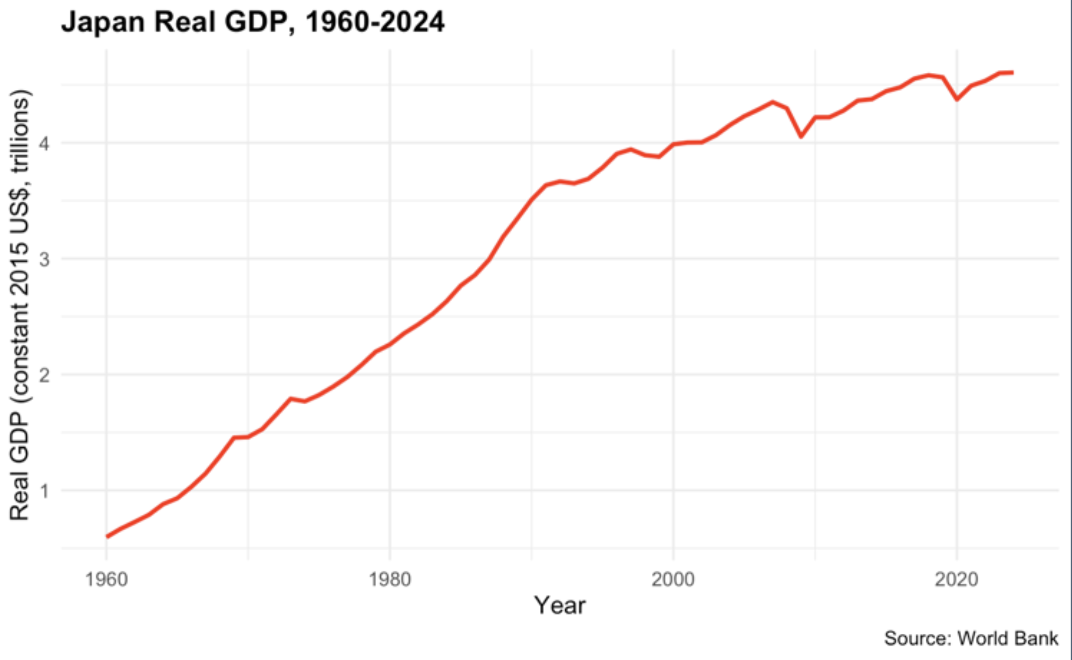
Figure 1: Japan’s real GDP shows rapid expansion until 1990, followed by significantly slower growth after the asset bubble collapse.
This graph highlights long-run growth trends. Real GDP increased sharply from under $1 trillion in 1960 to over $3 trillion by 1990, reflecting Japan’s high-growth period. After the bubble burst in the early 1990s, GDP continued to grow but at a much slower pace, eventually leveling off around $4–4.5 trillion. This shift marks the transition from rapid expansion to long-term stagnation.
Dataset source: World Bank
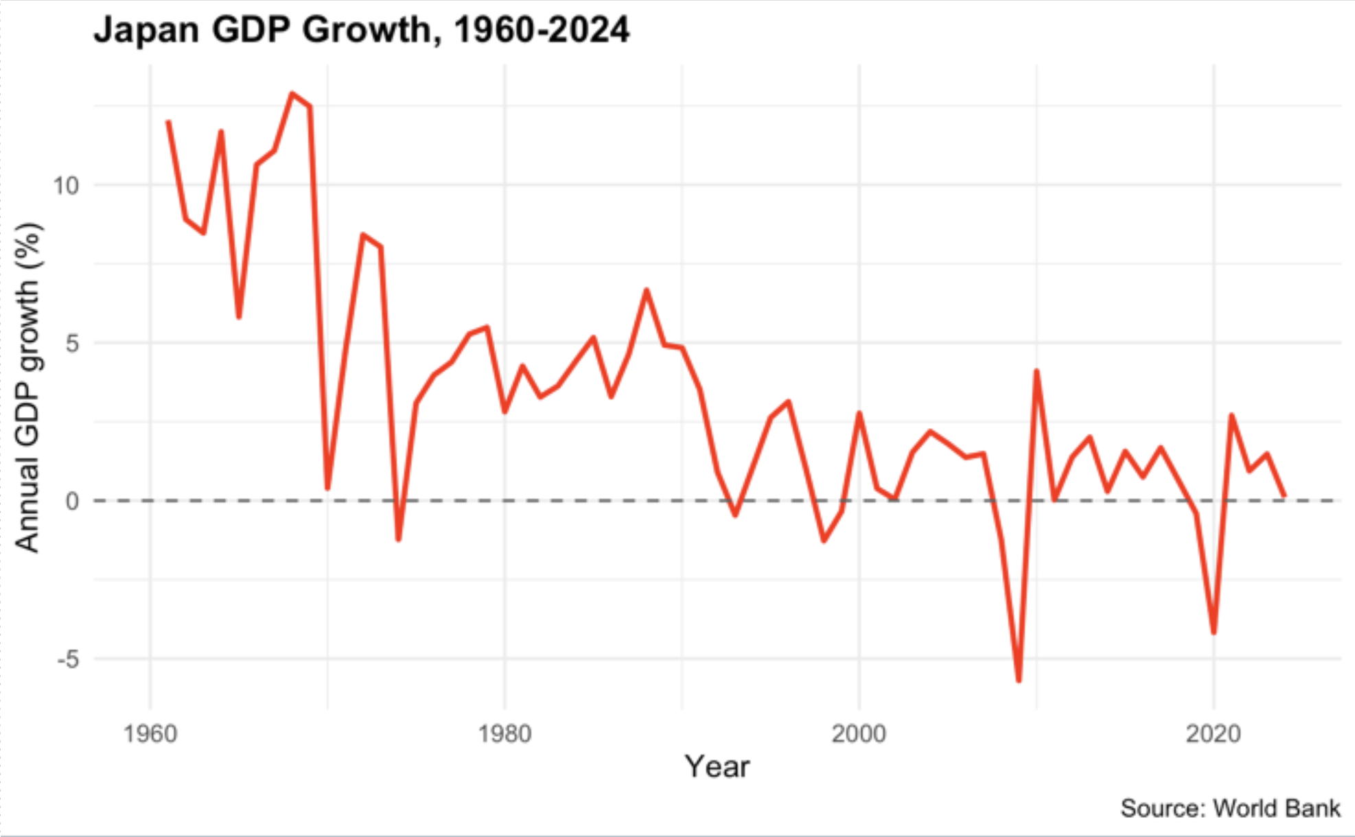
Figure 2: Japan’s GDP growth rates declined from double-digit levels in the 1960s to near-zero growth after the 1990s.
This graph captures changes in growth over time. Japan experienced very high growth rates in the 1960s, which gradually declined through the 1970s and 1980s. After 1990, growth became volatile and much lower, with several periods of negative growth. This reflects the end of Japan’s high-growth era and the persistence of economic stagnation following the asset bubble collapse.
Dataset source: World Bank
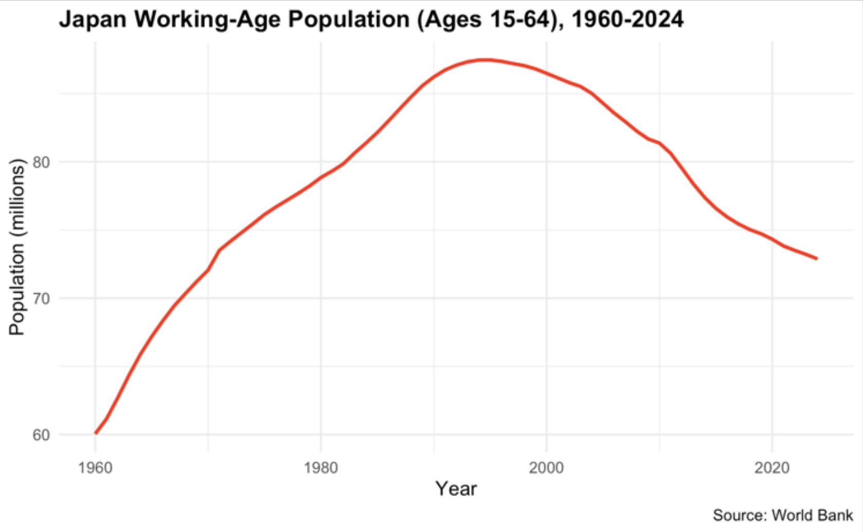
Figure 3: Japan’s working-age population grew steadily until the mid-1990s and has declined since, contributing to slower economic growth.
This graph shows labor force trends. The working-age population increased from about 60 million in 1960 to a peak of around 95 million in the mid-1990s, supporting strong economic growth. Since then, the population has declined to roughly 73 million, reflecting demographic aging and a shrinking labor force. This decline has reduced overall output and contributed to Japan’s long-term economic stagnation.
Dataset source: World Bank